Calculating the cross-sectional area of a stream
For this guide, we’ll take two approaches for calculating the area: one for non-georeferenced data (i.e., just a table with your measurements, as seen in testxs), and one for georeferenced data (made by sf).
Non-georeferenced data
Suppose you have a dataset like that which exists in testxs:
library(excess)
library(dplyr)
#>
#> Attaching package: 'dplyr'
#> The following objects are masked from 'package:stats':
#>
#>     filter, lag
#> The following objects are masked from 'package:base':
#>
#>     intersect, setdiff, setequal, union
library(ggplot2)
library(units)
#> udunits database from /usr/share/xml/udunits/udunits2.xml
head(testxs)
#> # A tibble: 6 × 3
#>   TAPE InvertRod Bankful
#>   [ft]      [ft]    [ft]
#> 1 0        -0.83   -3.29
#> 2 1        -1.01   -3.29
#> 3 3        -1.48   -3.29
#> 4 4.7      -1.19   -3.29
#> 5 5.95     -1.19   -3.29
#> 6 9.8      -1.93   -3.29
You’ll notice that the data has linear units listen in [ft]. This comes from the units package. Units of measurement aren’t necessary – the functions work fine without them – but it’s definitely good practice to ensure you’re calculating accurate results!
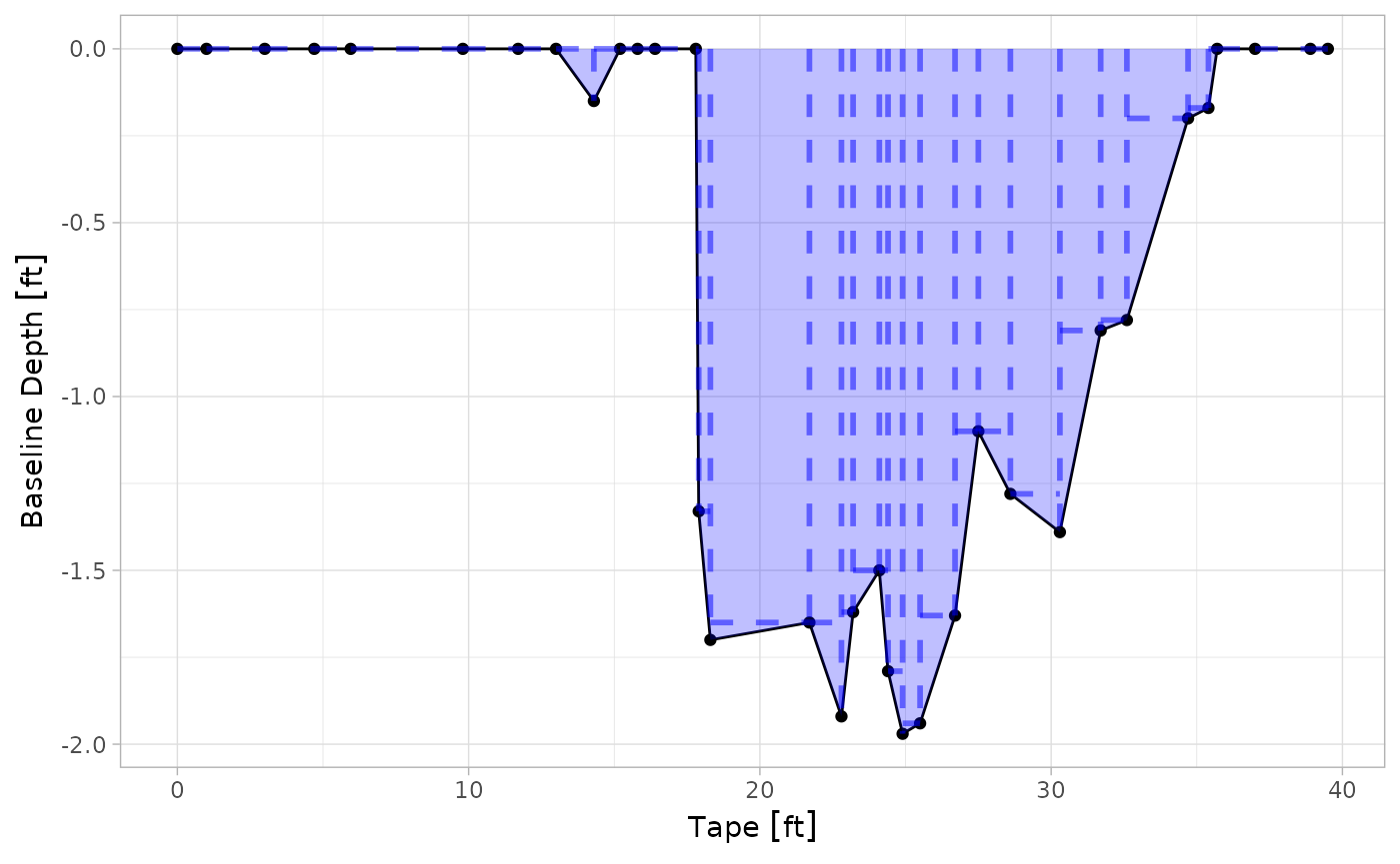
Anyways, we wish to calculate the cross-sectional area of the stream, and we have both the “x coordinate” (TAPE) and the “z-coordinate” (InvertRod). The Bankful column represents the bankful height, which is the “reference” for the depth measurement.
To calculate the cross-sectional area, excess uses the Trapezoidal Rule:
The trapezoidal area can be defined as:
\[A = \frac{1}{2} (x_n - x_{n-1})(y_n + y_{n-1})\]
For an implementation in R, we can use the dplyr::lag() and dplyr::lead() functions.